HOM & threshold detection

This example aims to demonstrate Hong-Ou-Mandel interference, the limitations of detection on Artemis and a technique for countering this.

import lightworks as lw
from lightworks import emulator, remote

try:
    remote.token.load("main_token")
except remote.TokenError:
    print(
        "Token could not be automatically loaded, this will need to be "
        "manually configured."
    )

HOM

Hong-Ou-Mandel interference is the foundational effect of photonic quantum computing. It occurs when indistinguishable photons are incident of a beam splitter, at which point an interference occurs and generates entanglement. The simplest case of this is when two photons are incident on different inputs of a 50:50 beam splitter. In this case the photons will always go to the same output as each other, and they end up in the superposition state \(\ket{2,0} + \ket{0, 2}\). This is contrary to what would be expected for classical light, where a \(\ket{1, 1}\) component would be measured 50% of the time. This is summarised in the image below.

Simulation

We can see the effect in Lightworks using the following circuit.

hom_circ = lw.PhotonicCircuit(2)
hom_circ.bs(0)

hom_circ.display()

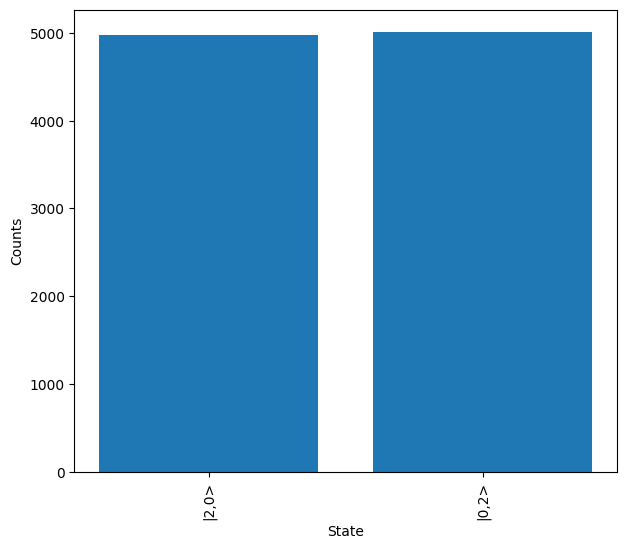
This is then sampled from, and as expected only \(\ket{2, 0}\) & \(\ket{0, 2}\) are measured.

sampler = lw.Sampler(hom_circ, lw.State([1, 1]), 10000)

backend = emulator.Backend("slos")

results = backend.run(sampler)
results.plot()

On Artemis, however, the detectors are single photon detectors and therefore can only indicate the presence of up to 1 photon per mode. This is sometimes known as threshold detection. We can simulate the effect of this using the detector module of the emulator.

sampler.detector = emulator.Detector(photon_counting=False)

backend = emulator.Backend("slos")

results = backend.run(sampler)
results.plot()

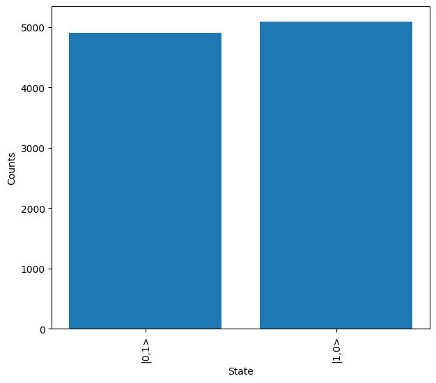
As can be seen above, now \(\ket{1,0}\) & \(\ket{0,1}\) are measured instead of \(\ket{2,0}\) & \(\ket{0,2}\). However the 1-photon states could correspond to either 1 or 2-photons at the output, meaning we cannot normally distinguish between photon loss and HOM interference effects.

Pseudo-PNR detection

There is a technique, however, called pseudo Photon-Number Resolving (PNR) detection which can be implemented to reduce the effect of this limitation. This comes at the cost of requiring an additional measurement mode per photon that needs to be measured. It is also a probabilistic effect so will reduce the number of measured output counts.

To achieve the desired affect, each output of the circuit is split into multiple modes using beam splitters, with the aim of dividing any-multi photon input states on a mode. In the case of 2 modes, a 50% beam splitter is found to be optimal. When using this, 50% of the time photons will go to different outputs after passing through the beam splitter, in which case they can then be resolved.

A circuit to observe the HOM effect through pseudo-PNR is created. The beam splitter on which HOM occurs is placed across modes 1 & 2, and then the additional beam splitters for the PNR detection are introduced.

thresh_circ = lw.PhotonicCircuit(4)

thresh_circ.bs(1, reflectivity=0.5)
thresh_circ.bs(0)
thresh_circ.bs(2)

thresh_circ.display()

In the circuit above, up to 2 photons can be measured. However, we can add additional beam splitters to further increase the number of photons that can be measured or increase the probability of success for a particular photon number. For 2 photons, the chance of success increases to 66.6% when using 3 modes. It can be seen below how the reflectivities in this case are 1/3 & 1/2, these are the optimal values for 3 modes. For each additional layer of beam splitters (mode), the optimal reflectivity of that layer will always be 1/n where n is the number of modes. So for 4 measurement modes, the optimal values will be 1/4, 1/3 & 1/2.

thresh_circ = lw.PhotonicCircuit(6)

thresh_circ.bs(2, reflectivity=0.5)
thresh_circ.bs(1, reflectivity=1 / 3)
thresh_circ.bs(3, reflectivity=1 / 3)
thresh_circ.bs(0)
thresh_circ.bs(4)

thresh_circ.display()

As this is significantly smaller than the size of the Artemis processor, we’ll choose to use this 6 mode version.

A sampler is then created, using the input state required for the HOM interference. The minimum detection is set to 2 so that we only get a valid measurement when the PNR detection is successful.

sampler = lw.Sampler(
    thresh_circ, lw.State([0, 0, 1, 1, 0, 0]), 10000, min_detection=2
)

This is then run on the backend and plotted below.

backend = remote.QPU("Artemis")

job = backend.run(sampler)

job.wait_until_complete()

results = job.get_result()
results.plot()

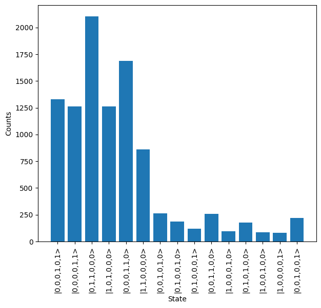
From this plot, it is hard to see the true results due the pseudo-PNR detection, so we’ll define a mapping which sums the photon counts across the combined detection modes and use the result remapping feature to then plot this data.

def mode_grouping(s: lw.State, n: int) -> lw.State:
    """
    Sum the first half of modes and second half and returns this as a 2 mode
    state.
    """
    return lw.State([sum(s[:n]), sum(s[n:])])


n = 3

m_results = results.map(mode_grouping, n=n)
m_results.plot()

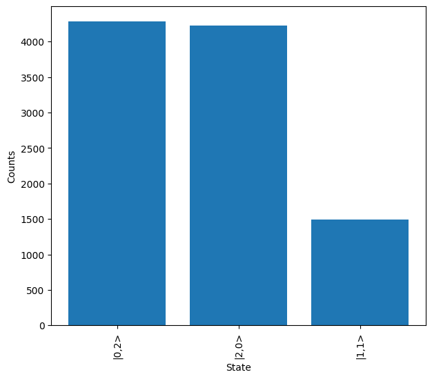
As expected, the 2 photon state is now observed a significant majority or the time.

Note

Due to the non-unity success rate of pseudo-PNR detection, the counts of the \(\ket{2, 0}\) & \(\ket{0, 2}\) states will be suppressed compared to \(\ket{1, 1}\). Some care should be taken when interpreting or processing data found with this method.