Quantum tomography

This example demonstrates how Lightworks can be used to be perform quantum state and process tomography on actual hardware.

import lightworks as lw
from lightworks import qubit, remote, tomography

import matplotlib.pyplot as plt
import numpy as np

try:
    remote.token.load("main_token")
except remote.TokenError:
    print(
        "Token could not be automatically loaded, this will need to be "
        "manually configured."
    )

State tomography

State tomography enables the density matrix of an output quantum state to be calculated.

To perform State tomography, an experiment function needs to be defined which takes a list of circuits to run and returns a list of Results. It can optionally feature additional arguments which are used for generalisation of the functions. The experiment function should contain all logic required for the creation of tasks and execution on a backend, below this includes defining the input_state and post-selection, as well as compiling all tasks into a batch for execution. A batch is used as it enables all tasks to be submitted at the same time, meaning they are all placed in the queue, and as it simplifies management of job status and downloading of results. The batch job is also saved to file to ensure this can be recovered in the event the program is interrupted and a load data option is included to automatically load existing jobs. Once all jobs are completed, the results from these are returned in a list, which should match the order that the circuits were provided to the function.

def run_state_tomo(
    experiments: list,
    n_qubits: int,
    job_name: str,
    load_data: bool = False,
) -> list:
    """
    Experiment function which is required for performing state tomography on a
    system. It takes a list of circuits and generates a corresponding list of
    results for each of them.
    """
    if not load_data:
        # Post-select on 1 photon across each pair of qubit modes
        post_select = lw.PostSelection()
        for i in range(n_qubits):
            post_select.add((2 * i, 2 * i + 1), 1)
        # Start in all 0 state
        input_state = lw.convert.qubit_to_dual_rail("0" * n_qubits)
        # Create a batch of jobs to submit
        batch = lw.Batch(
            lw.Sampler,
            task_args=[experiments.all_circuits, [input_state], [100000]],
            task_kwargs={"post_selection": [post_select]},
        )
        # Generate QPU backend and run batch
        backend = remote.QPU("Artemis")
        jobs = backend.run(batch, job_name=job_name)
        # Save in case these need to be recovered later
        jobs.save_to_file(job_name, allow_overwrite=True)
    else:
        jobs = remote.load_job_from_file(job_name)
    # Once jobs are complete then return results
    jobs.wait_until_complete()
    return list(jobs.get_all_results().values())

To start, we’ll look at the \(\ket{+} = \frac{1}{\sqrt{2}}(\ket{0}+\ket{1})\) state, which can be generated by applying the hadamard gate to \(\ket{0}\). This circuit can be created using the built-in gate.

h_gate = qubit.H()

h_gate.display()

The tomography can then be performed with the StateTomography object from Lightworks. With this, the experiments are generated which can then be use with the run function earlier to automatically submit these and retrieve results.

Note

The load data option is omitted here. If you need to recover jobs which have already been submitted then this can be achieved by adding True to experiment_args, so the new value would be [n_qubits, "plus_state_tomography", True].

n_qubits = 1

tomo = tomography.StateTomography(
    n_qubits,
    h_gate,
)
experiments = tomo.get_experiments()

results = run_state_tomo(experiments, n_qubits, "plus_state_tomography")

These results are then passed to the process method, in this case we’ll use the projection option to ensure the calculated density matrix is physical.

rho = tomo.process(results, project_to_physical=True)

This can then be plotted against the expected density matrix. This is defined as \(\rho = \ket{\psi}\bra{\psi}\), so for the expected state \(\ket{+}\) we find:

\begin{equation}\rho = \ket{+}\bra{+} = \begin{bmatrix} 0.5 & 0.5\\ 0.5 & 0.5 \end{bmatrix}\end{equation}

This can be calculated from Lightworks by providing the vector representation of the state to the density_from_state function. For \(\ket{+}\) the vector representation is \(\frac{1}{\sqrt{2}}\cdot\begin{bmatrix} 1\\ 1 \end{bmatrix}\)

rho_exp = tomography.density_from_state([2**-0.5, 2**-0.5])

The plots can then be created.

# Find plot range
vmin = min(
    a.min()
    for a in [np.real(rho), np.imag(rho), np.real(rho_exp), np.imag(rho_exp)]
)
vmax = max(
    a.max()
    for a in [np.real(rho), np.imag(rho), np.real(rho_exp), np.imag(rho_exp)]
)

# Create figure
fig, ax = plt.subplots(2, 2, figsize=(12, 10))
ax[0, 0].imshow(np.real(rho), vmin=vmin, vmax=vmax)
ax[0, 0].set_title("Re(\u03c1)")
ax[0, 1].imshow(np.imag(rho), vmin=vmin, vmax=vmax)
ax[0, 1].set_title("Re(\u03c1)")
ax[1, 0].imshow(np.real(rho_exp), vmin=vmin, vmax=vmax)
ax[1, 0].set_title("Expected Re(\u03c1)")
im = ax[1, 1].imshow(np.imag(rho_exp), vmin=vmin, vmax=vmax)
ax[1, 1].set_title("Expected Im(\u03c1)")
fig.colorbar(im, ax=ax.ravel().tolist())

# Set ticks as integer values and create state labels
ticks = range(rho.shape[0])
n_qubits = int(np.log2(len(ticks)))
basis = ["0", "1"]
labels = list(basis)
for _ in range(n_qubits - 1):
    labels = [q1 + q2 for q1 in labels for q2 in basis]
for i in range(2):
    for j in range(2):
        ax[i, j].set_xticks(ticks, labels=labels)
        ax[i, j].set_yticks(ticks, labels=labels)

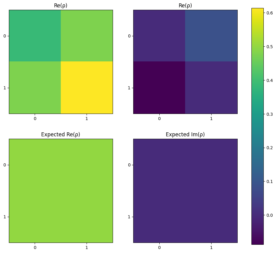
It is also possible to evaluate the fidelity of state generation using state_fidelity.

f = tomography.state_fidelity(rho, rho_exp)
print(f"Fidelity = {round(f * 100, 2)} %")

Fidelity = 97.9 %

Process tomography

Process tomography can be used to gain an understanding of the actual operation implemented by a quantum processor.

One form of process tomography is the calculation of average gate fidelity. To achieve this, the following equation can be used [Nie02]:

\(\begin{equation}\overline{F}(\mathcal{E}, U) = \frac{\sum_{jk}\alpha_{jk}tr(UU_j^{\dagger}U^{\dagger}\mathcal{E}(\rho_k))+d^2}{d^2(d+1)}\end{equation},\)

In the same way as with state tomography, an experiment function should be defined - this time accepting a list of circuits and a list of input states.

def run_process_tomo(
    experiments: list,
    n_qubits: int,
    job_name: str,
    load_data: bool = False,
) -> list:
    """
    Experiment function which is required for performing process tomography on a
    system. It takes a list of circuits and generates a corresponding list of
    results for each of them.
    """
    if not load_data:
        # Post-select on 1 photon across each pair of qubit modes
        post_select = lw.PostSelection()
        for i in range(n_qubits):
            post_select.add((2 * i, 2 * i + 1), 1)
        # Create a batch of jobs to submit
        batch = lw.Batch(
            lw.Sampler,
            task_args=[
                experiments.all_circuits, experiments.all_inputs, [25000]
            ],
            task_kwargs={"post_selection": [post_select]},
        )
        # Generate QPU backend and run batch
        backend = remote.QPU("Artemis")
        jobs = backend.run(batch, job_name=job_name)
        # Save in case these need to be recovered later
        jobs.save_to_file(job_name, allow_overwrite=True)
    else:
        jobs = remote.load_job_from_file(job_name)
    # Once jobs are complete then return results
    jobs.wait_until_complete()
    return list(jobs.get_all_results().values())

Again, we’ll look at the hadamard gate which is re-defined below.

h_gate = qubit.H()

h_gate.display()

As part of the gate fidelity calculation, the unitary for the expected process needs to be defined. For the Hadamard this is:

\begin{equation} \text{U}_\text{H} = \frac{1}{\sqrt{2}}\begin{bmatrix} 1 & 1 \\ 1 & -1 \end{bmatrix},\end{equation}

target_process = 1 / 2**0.5 * np.array([[1, 1], [1, -1]])

The tomography can then run to compute the fidelity from the target system.

n_qubits = 1

tomo = tomography.GateFidelity(n_qubits, h_gate)
experiments = tomo.get_experiments()

results = run_process_tomo(experiments, n_qubits, "H_process_tomography")

The results are again processed, using a projection to ensure the result is physical.

avg_fidelity = tomo.process(results, target_process, project_to_physical=True)
print(f"Average gate fidelity = {avg_fidelity * 100} %")

Average gate fidelity = 97.8949410082671 %

Next steps

It should now be possible for you to perform benchmarking of a range of quantum gates. The code above is intended to be mostly generalised, meaning it should be a simple process to switch to different target states/processes.