Boson sampling

Boson sampling was first proposed in [AA10] as a near-term way of demonstrating quantum advantage, primarily targetted at photon systems. This is possible as calculating the output probability distribution of n-photons into a linear interferometer requires calculation of the permanent of the unitary which is programmed into the interferometer. The calculation of the permanent is #P-hard, marking this very expensive to compute classically for larger systems.

Artemis consists of a multi-photon input generator and a universal interferometer, making it ideal for testing this approach to quantum computing.

import lightworks as lw
from lightworks import remote

import matplotlib.pyplot as plt
import numpy as np

try:
    remote.token.load("main_token")
except remote.TokenError:
    print(
        "Token could not be automatically loaded, this will need to be "
        "manually configured."
    )

Setup

To demonstrate boson sampling on the system, we’ll start by generating a random 20 x 20 unitary. There is an included function within Lightworks for this.

unitary = lw.random_unitary(20, seed=111)

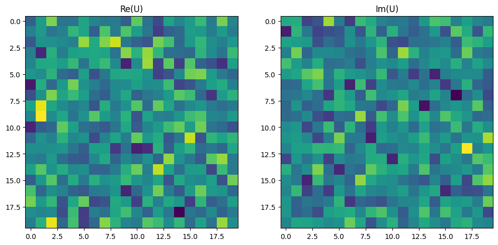
Plotting this unitary, it can be seen how it has a real and imaginary component, both of which are distributed across all inputs and outputs of the interferometer (i.e. it is not a sparse matrix).

fig, ax = plt.subplots(1, 2, figsize=(12, 6))

ax[0].imshow(np.real(unitary))
ax[0].set_title("Re(U)")
ax[1].imshow(np.imag(unitary))
ax[1].set_title("Im(U)")
plt.show()

This matrix can then be converted into a circuit using the Unitary object.

circuit = lw.Unitary(unitary)

We’ll then define an input state, in this case a 3-photon state is configured, with photons on modes 2, 6, & 10.

input_modes = [2, 6, 10]

input_state = lw.State(int(i in input_modes) for i in range(circuit.n_modes))
print(input_state)

|0,0,1,0,0,0,1,0,0,0,1,0,0,0,0,0,0,0,0,0>

Finally, the circuit and input state are collected in a sampling task. The value of min_detection is set to 4 (also the number of input photons) to mitigate the effects of photon loss in the system.

sampler = lw.Sampler(circuit, input_state, 1000, min_detection=3)

Results

This job can then be executed and the results retrieved.

qpu = remote.QPU("Artemis")

job = qpu.run(sampler)

job.wait_until_complete()

results = job.get_result()

Once complete, we’ll attempt to visualize the results. Due to the size and complexity of these states, the built-in plotting method is not particularly helpful in this case. Instead, we’ll sum the number of photons measured on each mode and plot this as a Histogram.

mode_counts = [0] * circuit.n_modes

for state, count in results.items():
    for mode, n_photon in enumerate(state):
        mode_counts[mode] += n_photon * count

plt.bar(range(circuit.n_modes), mode_counts)
plt.xlabel("Mode")
plt.ylabel("Photon counts")
plt.show()